Understanding Surfaces
The 3D version of connect-the-dots is more advanced than the 2D version and aims to create a 3D model instead of just lines. Civil 3D 2025 achieves this using a computer algorithm called the Triangular Irregular Network (TIN) algorithm.
The TIN algorithm connects each point to at least two neighboring points using 3D lines. This results in a triangular spider web-like structure, with triangles of various shapes and sizes due to the irregular spacing between points. The “T” in TIN stands for triangles, the “I” for irregular, and the “N” for the network formed by connected points and lines.
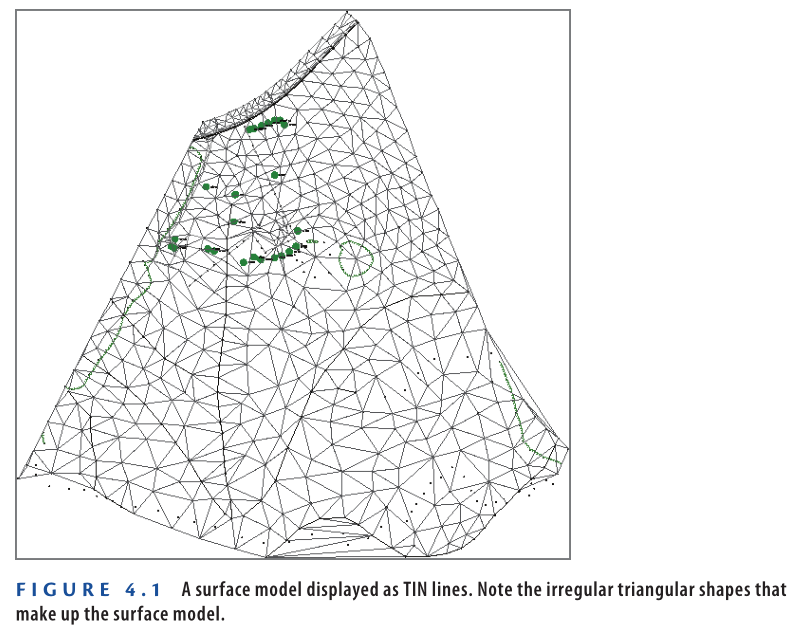
The triangles in a TIN model are just a visual representation of the algorithm, but the real power lies in its ability to calculate elevations for any point within the model. Even if a point is inside a triangle, its elevation can still be determined. This ability makes the TIN model a true 3D model. It can be virtually sliced, rotated, filled, excavated, or used for water flow simulations. These capabilities make surface models integral to the functionality of Civil 3D 2025.
Creating a Surface from Survey Data
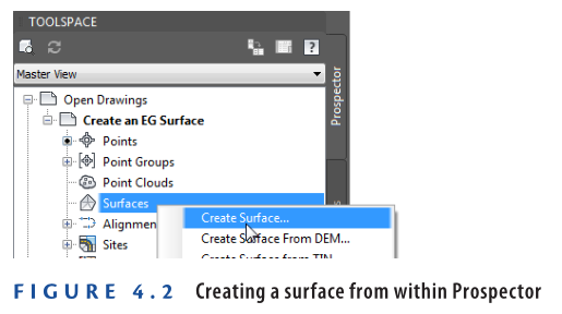
To create a surface in Civil 3D 2025, navigate to the Prospector tab, right-click the Surfaces node in the tree, and select Create Surface, as shown in Figure 4.2. The surface will immediately appear in Prospector but won’t be visible in the drawing until data is added. Surfaces are fundamentally composed of points and lines. You provide the source of the points, and Civil 3D generates the connecting lines. In this stage, survey points are typically used as the initial source for surface-point data.
Exercise 4.1: Create an Existing Ground Surface
In this exercise, you’ll create a surface using survey data:
- Open the drawing named Create an EG Surface.dwg, located in the Chapter 04 class data folder.
- In Prospector, right-click on Surfaces and select Create Surface.
- In the Create Surface dialog box, enter EG in the Name field.
- For Style, select C-Existing Contours (1′) or C-Existing Contours (0.5 m), depending on your preferred units. Click OK to close the Create Surface dialog box.
- In Prospector, expand Surfaces ➢ EG ➢ Definition. Review the items listed beneath EG in the tree, as shown in Figure 4.3.
Components of a Surface
As shown in Figure 4.3, various types of information can define and shape a surface. Below is a brief description of each component:
- Boundaries: Define the limits of the surface. Boundaries can enclose the surface within a specific area or exclude interior regions, such as ponds or buildings.
- Breaklines: Align TIN lines with linear features, defining hard edges like embankments, curbs, or ditches.
- Contours: Typically seen as the final output of a surface, contours can also serve as input data to define a surface.
- DEM Files: Digital Elevation Models are large-scale, low-accuracy datasets used for rough analysis or calculations.
- Drawing Objects: AutoCAD entities like lines, blocks, and text can define a surface if created at the correct elevations.
- Edits: Modifications to enhance surface accuracy or usability. Editing methods will be covered in this chapter.
- Point Files: Text files containing x, y, and z data can be imported directly into a surface without creating Civil 3D points.
- Point Groups: Allow for simultaneous selection of multiple points. Point groups are a common method to define a surface in Civil 3D.
- Point Survey and Figure Survey Queries: Advanced tools from survey functionality for selecting points and figures based on survey properties. These are not covered in this book but are detailed in Civil 3D help content.
6: Right-click Point Groups under the EG ➢ Definition tree and select Add.
7: Select Ground Shots from the list, then click OK.
- The surface will now be visible in the plan view as contours and shaded 3D faces in the bottom-right 3D viewport.
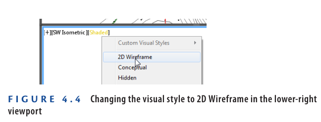
8: In the lower-right viewport, click on Shaded and change the view style to 2D Wireframe, as shown in Figure 4.4.
- The surface appearance will update to display the TIN lines.
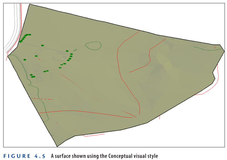
9: In the lower-right viewport, click 2D Wireframe and select Conceptual from the dropdown menu.
- To orbit the view, hold the Shift key and click and drag the center mouse button.
- Observe the surface from multiple viewpoints to examine its 3D features.
10: Save and close the drawing.
- To review the completed exercise, open Create an EG Surface – Complete.dwg.
https://www.mediafire.com/file/plgqq4u1s692xco/Create+an+EG+Surface+-+Complete.dwg/file
Watch Complete Video here for this Exercise:
Using Breaklines to Improve Surface Accuracy
The TIN algorithm connects the closest points with 3D lines to create surfaces. However, this approach may not always yield the most accurate surface model. In such cases, the TIN lines need to be forced into a specific arrangement that matches linear features like curbs, embankments, or walls. Breaklines are used for this purpose.
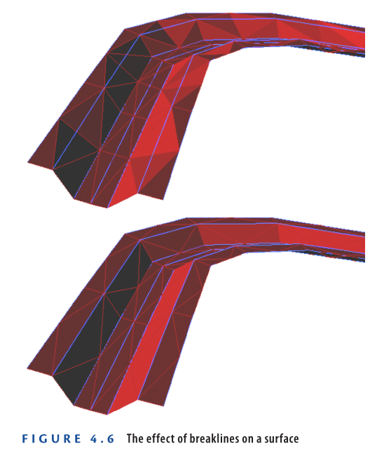
As shown in Figure 4.6, the blue lines represent the edges of a channel, while the TIN lines are red. In the top image, the blue lines are not included as breaklines, resulting in a rough and inaccurate channel representation. In the bottom image, breaklines force the TIN lines to align with the channel edges, creating a smoother and more accurate surface model.
Adding Breaklines to a Surface
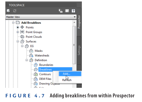
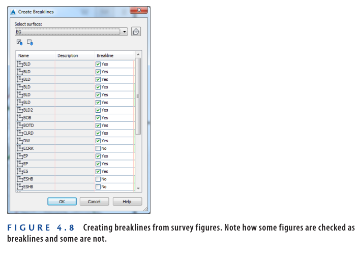
From Prospector, you can add breaklines by right-clicking the Breaklines node for a specific surface and selecting Add (see Figure 4.7). For survey data, there is an even simpler method. From the Survey Toolspace, right-click Figures and select Create Breaklines. This opens a list of all your survey figures, some of which are checked as breaklines while others are not (see Figure 4.8).
How does the command determine which figures are breaklines? This is based on the figure prefix database discussed in Chapter 3. When the figures were created, they were automatically classified as breaklines or non-breaklines according to the code assigned to the points defining them.
Exercise 4.2: Add Breaklines
In this exercise, you’ll add breaklines to a surface and observe their effect on the accuracy of the surface.
- Open the drawing named Add Breaklines.dwg which you can download from Youtube video description below.
- On the Survey tab of the Toolspace, right-click Survey Databases and select Set Working Folder.
- Browse to and select the Chapter 04 class data folder. Click OK.
You should see a different survey database named Essentials. - Right-click the Essentials survey database, and select Open For Edit.
- Expand the Essentials database. Right-click Figures, and select Create Breaklines.
- Scan the list of figures, and note which ones are tagged as breaklines. Click OK.
- In the Add Breaklines dialog box, change the Mid-Ordinate Distance value to 0.03, and click OK.
Breaklines in the Field
Breaklines are linear features that mark a change in the slope of the ground. As you study the list of figures in this exercise, you might wonder why some are designated as breaklines while others are not.
Some breaklines are quite obvious, such as a set of bottom of bank (BOB) points or top of ditch (TOPD) points. Others serve double duty, like an edge of pavement (EP). This survey figure indicates the line where pavement ends and dirt begins. However, there is typically a change in slope at this line between the slope of the ground and the manmade slope of the road. For this reason, EPs are often tagged as breaklines.
On the other hand, features like a right of way (ROW), treeline (TL), or fence line (FENC) obviously have nothing to do with the slope of the ground; therefore, they are not checked as breaklines.
You should notice a change in the contours along the red breaklines. These breaklines define the swales, edges, and ridges that were recognized in the field and explicitly located as terrain features. Additionally, notice that contours now cover the road area to the north, where the surface is made strictly of breaklines.
- In the top-right viewport, click one of the surface contours, and then click Surface Properties on the ribbon.
- On the Information tab of the Surface Properties dialog box, change Surface Style to Triangles. Click OK and press Esc to clear the selection of the surface.
- Notice how TIN lines don’t cross the breaklines.
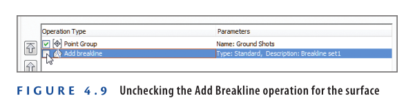
- Select the surface and open Surface Properties again. On the Definition tab, uncheck the box next to Add Breakline, as shown in Figure 4.9. Click OK, and then click Rebuild The Surface.
You have removed the effect of the breaklines temporarily. Notice how the TIN lines now cross back and forth over the swale and ridge lines, creating a rough edge where there should be a sharp, well-defined edge.
- Repeat step 10, but this time check the box next to Add Breakline. The breaklines are once again applied to the surface.
- Save and close the drawing.
You can view the results of successfully completing this exercise by opening Add Breaklines – Complete.dwg.
https://www.mediafire.com/file/4sr5z9drfmd9jka/Add+Breaklines+-+Complete.dwg/file
Watch Complete Video here for this Exercise:
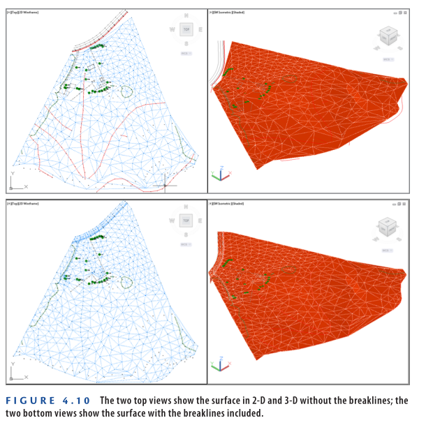
This exercise highlights the importance of breaklines. Simply connecting a set of points with 3D triangular shapes does not always generate an accurate surface. In specific areas, the shapes need to be adjusted so they align with terrain features, accurately modeling their form. Figure 4.10 compares the surface with and without breaklines in both 2D and 3D views.
Breakline Settings and Options
The Add Breaklines dialog box offers several options and values. Here’s a brief explanation of the key settings:
Type
Among the five types available, the most relevant to discuss are Proximity and Standard:
- Standard Breaklines:
- Alignment of TIN Lines: Standard breaklines control the alignment of TIN lines, as previously discussed.
- Additional Point Information: Their vertices serve as a source of extra point data for the surface.
- Since only the Ground Shots point group has been added to the surface, it’s crucial that points accompany any breaklines you add.
- For this to work correctly, the vertices of the breaklines must be 3D and set to the correct elevations.
Proximity Breaklines
Proximity breaklines control only the alignment of TIN lines. Unlike standard breaklines, they can be 2D. However, they rely on nearby points to “steal” their elevations.
- If all survey points were added to your surface, the survey figures could have been added as proximity breaklines.
Weeding Factors
Sometimes breaklines contain too many vertices, potentially overloading the surface with data.
- Weeding is the selective removal of points based on distance and angle, reducing unnecessary complexity in the surface.
Supplementing Breaklines
- By Distance:
- Long stretches of breaklines without vertices can result in reduced accuracy because TIN lines are generated only at points.
- When you enable the Distance option, Civil 3D adds more points along the breakline, spaced at intervals you define.
- By Mid-Ordinate:
- Curves in breaklines are approximated by a series of short TIN lines since TIN lines are straight.
- The Mid-Ordinate value determines how closely these short lines follow the curve:
- A smaller mid-ordinate value (e.g., 0.1) results in shorter, more numerous TIN lines, improving surface accuracy.
- A larger mid-ordinate value (e.g., 1.0) creates fewer TIN lines, reducing detail.
- This method works well across a wide range of curve radius.
Editing Surfaces
With the inclusion of points and breaklines, you’ve provided most of the data required to create a surface model. However, further refinement is necessary to achieve the most accurate representation of the existing ground surface. Surface editing can be done in several ways. Below, we discuss three key methods: adding boundaries, deleting lines, and editing points.
Adding Boundaries
Boundaries define where the surface exists and where it does not. For example, in a project, you might not want the surface to extend outside the surveyed area.
Why Prevent Surface Extension?
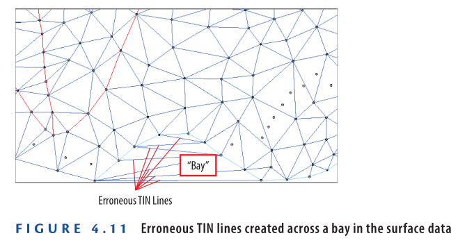
If the edge of a point-represented area bends inward, the lines forming the surface may extend across the “bay,” creating inaccurate surface data (see Figure 4.11).
Solution: Outer Boundary
To avoid or correct this issue, an outer boundary is applied to prevent the surface from existing in such areas. This ensures the surface model remains accurate and contained within the surveyed region.
Another common issue with surface models is when they extend into areas they shouldn’t, such as the footprint of a building. It is considered poor drafting practice to display contours passing through a building since the ground surface is not accessible in that location.
Hide Boundary
A hide boundary is a type of boundary that removes surface data within a specified area, creating a void or “hole” in the surface.
- This ensures the surface does not appear in areas where it should not exist, such as within a building’s footprint.
Types of Boundaries
Civil 3D offers four types of boundaries to manage surface data effectively:
- Outer
- An outer boundary establishes a perimeter for the surface.
- No surface data can exist outside an outer boundary.
- This type of boundary is commonly used in most surfaces.
- Hide
- A hide boundary creates a void, or “hole,” in the surface.
- Hide boundaries are used to remove surface data within buildings or other unwanted areas.
- Show
- A show boundary creates an island of data within a hide boundary.
- For example, a courtyard within the footprint of a building can be defined using a show boundary.
- Data Clip
- Unlike the first three types, a data-clip boundary prevents data outside it from ever becoming part of the surface.
- Data-clip boundaries are used when creating a small surface from source data that covers a large area.
Exercise 4.3: Add Boundaries
In this exercise, you’ll add boundaries around the buildings that will remove surface data from within their footprints.
- Open the drawing named Surface Boundaries.dwg which you can download from Youtube video description below.
- Click one of the surface contours in the top-right viewport. Then, on the Tin Surface: EG tab of the ribbon, click Add Data ➢ Boundaries.
- Enter Bld1 as the boundary name, and select Hide as the type. Make sure the box next to Non-Destructive Breakline is checked, and click OK.
- Select one of the buildings in the top-right viewport, and press Enter. You should immediately see a hole appear in the surface shown in the lower-right viewport. If you’ve selected a building with contours running through it, you’ll see the contours disappear in the upper-right viewport. It appears that they have been trimmed, but actually, the surface data has been removed from within the shape of the building.
5. Repeat steps 2 to 4 for the other buildings, even if contours don’t pass through them. Use a name other than Bld1 or the software won’t accept your boundaries.
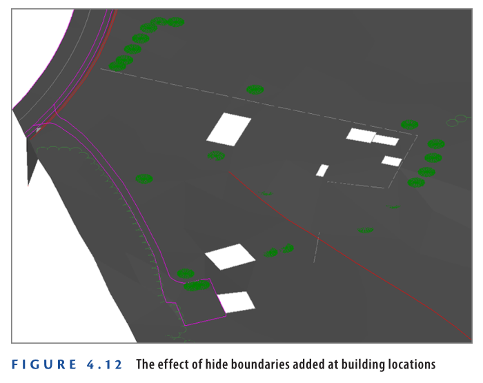
6. In the lower-right viewport, zoom in to the area of the buildings, and notice that there are now voids where the buildings are located, as shown in Figure 4.12.
7. Save and close the drawing.
You can view the results of successfully completing this exercise by opening
Surface Boundaries – Complete.dwg.
https://www.mediafire.com/file/liwh3lo9mnhxzd3/Surface+Boundaries+-+Complete.dwg/file
Watch Complete Video here for this Exercise:
Deleting lines
Another, less eloquent way of removing unwanted TIN lines is to delete them from the surface rather than use a boundary to do it for you. This method is best when you need to remove only a few TIN lines in isolated areas. There are two important things to remember when deleting TIN lines. First, in order for the lines to be deleted, they must be visible, which means you must apply a style that displays them. Second, you can’t use the AutoCAD ERASE command to remove them; instead, you must use the Delete Line command created specifically for surfaces.
Exercise 4.4: Delete lines
In this exercise, you’ll delete unwanted TIN lines from the surface.
- Open the drawing named Delete TIN Lines.dwg which you can download from Youtube video description below.
- Click one of the contours in the top-right viewport, and then select Surface Properties on the ribbon.
- On the Information tab, change Surface Style to Triangles and click OK. Press Esc to clear the selection of the surface.
- In the left viewport, zoom in to the southern edge of the surface, and note the TIN lines that extend across the bend in the stream (shown previously in Figure 4.11).
- Select one of the TIN lines, and then click Edit Surface ➢ Delete Line on the ribbon. Select the erroneous lines as indicated previously in Figure 4.11. Press Enter after you’ve made your selection.
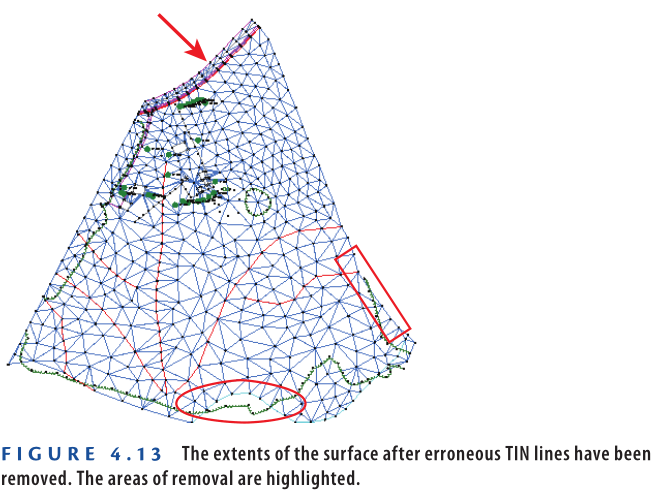
- Pan around the edge of the surface, and delete any other TIN lines that look like they don’t belong. The resulting surface should look similar to Figure 4.13.
7. Save and close the drawing.
You can view the results of successfully completing this exercise by opening Delete TIN Lines – Complete.dwg.
https://www.mediafire.com/file/tcrt7loevfrnqwy/Delete+TIN+Lines+-+Complete.dwg/file
Watch Complete video here for this Exercise:
Exercise 4.5: Edit Points
You have already learned about editing survey source data (survey points and survey figures). In this exercise, you’ll edit the surface.
- Open the drawing named Editing Points.dwg which you can download from Youtube video description below.
The two right viewports are zoomed in to the location where the driveway meets the road on the north side of the property. In this area, one of the surface points is incorrect. In the plan view on the top right, the effects of the incorrect point can be seen in the densely packed contours. In the 3-D view on the bottom right, the erroneous point appears as a downward spike in the surface. - Click one of the contours to select the surface, and then click Surface Properties on the ribbon.
- In the Surface Properties dialog box, click the Information tab and change Surface Style to Triangles And Points. Click OK.
The display of the surface changes to lines and points, with the points appearing as plus-sign markers. - Click any TIN line to select the surface, and then click Edit Surface ➢ Modify Point on the ribbon.
- When prompted to select a point, click the point in the 3-D view that is located well below the other points (see Figure 4.14). Press Enter.
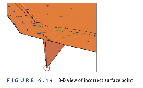
6. At the command line, type 190.76 (58.144), and press Enter.
Notice how the surface is modified but the survey figure is left behind. Depending on the situation, it may be prudent to go back to the source data for the survey figure and correct that as well.
7. Press Enter to exit the Modify Point command.
Change the style of the surface back to C-Existing Contours (1′) (C-Existing Contours (0.5 m)). Notice that the closely spaced contours in the top-right viewport are no longer there.
8. Save and close the drawing.
You can view the results of successfully completing this exercise by opening Editing Points – Complete.dwg.
https://www.mediafire.com/file/d2twufuf0vdwsnw/Editing+Points+-+Complete.dwg/file
Displaying and Analyzing Surfaces
Because you’re working with surface objects in Civil 3D, you can do much more than simply show contours. Civil 3D surfaces can help you tell many different stories about the shape of the land and how water will flow across it. They are able to do this through multiple types of analyses as well as the ability for styles to display analysis results in nearly any way you wish. With these tools at your disposal, you can study the terrain thoroughly and make smart choices about the direction of your design early in the process.
Analyzing Elevation
Elevation analysis allows you to delineate any number of elevation ranges and then graphically distinguish the different ranges by color. This is a useful tool in many instances, especially when you’re working with someone who doesn’t know how to read contours.
Exercise 4.6: Analyze Elevation
In this exercise, you’ll perform an elevation analysis on a surface in your drawing.
- Open the drawing named Elevation Analysis.dwg which you can download from Youtube video description below.
- Click one of the contours to select the surface, and then click Surface Properties on the ribbon.
- Change Surface Style to Elevation Banding (2-D).
- Click the Analysis tab. Verify that the analysis type is Elevations and the number of ranges is 8.
- Click the downward-pointing arrow to populate the Range Details section of the dialog box with new data.
- Click OK to return to the drawing. Press Esc to clear the selection of the surface.
The surface undergoes an obvious change, and it’s now displayed as a series of colored bands with red signifying the lowest elevations and purple signifying the highest. - Change the style of the surface to Elevation Banding (3-D).
Now the 3-D view displays the colored bands as a 3-D representation with exaggerated elevations. This tells a clear story about the existing shape of the land for this site (see Figure 4.15).

8. Save and close the drawing.
You can view the results of successfully completing this exercise by opening Elevation Analysis – Complete.dwg.
https://www.mediafire.com/file/lhwr2cdqcq8tsb3/Elevation+Analysis+-+Complete.dwg/file
Watch Complete Video here for this Exercise:
Analyzing Slope
Another important aspect of the terrain is the slope. Areas with very steep slopes are difficult to navigate either by construction vehicles or the eventual occupants of the property. Flat slopes are much more accessible, but if they are too flat, then drainage problems often occur. One of your tasks as a designer is to ensure that your project has the right slopes in the right areas. By studying the slopes of the existing topography, you can locate features where slopes are good or determine that terrain modifications will be necessary to create good slopes.
Civil 3D can display slopes in two ways. The first is to show the slopes as colored ranges like the ones you saw in the previous section. The second is to use slope arrows that can be color-coded to indicate what range they’re located in, with the added benefit of always pointing downhill to show you the direction of water flow.
Exercise 4.7: Analyze Slope
In this exercise, you’ll perform a slope analysis on a surface in your drawing.
- Open the drawing named Slope Analysis.dwg which you can download from Youtube video description below.
- Click one of the contours to select the surface, and then click Surface Properties on the ribbon.
- On the Information tab of the Surface Properties dialog box, change Surface Style to Slope Banding (3-D).
- Click the Analysis tab. Change Analysis Type to Slopes, and click the downward-pointing arrow.
- Click OK. Press Esc to clear the selection of the surface and zoom in to the 3-D view of the surface in the bottom-right viewport.
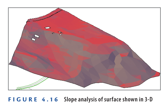
In the 3-D image on the bottom right, the darkest reds signify the steepest slopes. This enables you to see that the area north of the farm is fairly flat pasture land while the area to the south of the farm slopes dramatically toward the stream farther to the south (see Figure 4.16). - Access Surface Properties again, and change the style to Slope Arrows.
- On the Analysis tab, choose Slope Arrows as the analysis type, and click the arrow again.
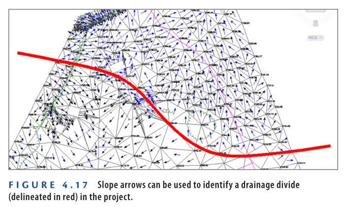
8: Click OK to return to the drawing. Press Esc to clear the selection of the surface. In this view, the darker blues and blacks represent the steepest slopes, and the arrows always point downhill. As you study the arrows, you should notice a drainage divide that runs west to east through the farm buildings; it’s delineated in red in Figure 4.17. Rainfall falling to the north of this area drains to the road, and rain falling south of it drains to the stream.
9: Save and close the drawing.
You can view the results of successfully completing this exercise by opening Slope Analysis – Complete.dwg.
https://www.mediafire.com/file/vz7twmoqdj7orwy/Slope+Analysis+-+Complete.dwg/file
Watch Complete video here for this Exercise:
Performing Other Types of Analysis
In addition to analyzing elevations, slopes, and slope arrows, you can perform the following types of analyses:
Contours
Contours can be used to analyze a surface. They can be color-coded, and you can create a legend table that shows the area and/or volume the contours represent.
Directions
With this type of analysis, you can see a visual representation of your surface slopes. For example, you can use the analysis to see which parts of your surface slope to the south and which slope to the north.
User-Defined Contours
Contours are usually placed at even intervals, such as the 1′ (0.5-meter) contours with which you have been working so far. What if you want to show a contour that represents elevation 92.75? That’s done as a user-defined contour. A user-defined contour is an individual instance of a contour, usually at an irregular interval.
Watersheds
A watershed analysis outlines areas within the surface where rainfall runoff flows to a certain point or in a certain direction. This type of analysis is yet another way of studying the drainage characteristics of the terrain.
Exploring Even More Analysis Tools
There are even more ways of analyzing your surface that aren’t found in Surface Properties. For example, the following tools are especially useful on many projects:
Water Drop Tool
With the Water Drop tool, you can click any point on your surface and Civil 3D will trace the downhill path of that point until it reaches a low point or encounters the edge of the surface. This is a very detailed way to study how water will flow across the ground.
Catchment Area Tool
With this tool, you can click a point on the surface and Civil 3D will draw a closed shape that represents the area that flows to that point. This is very useful when you’re analyzing the effects of rainfall on your project.
Quick Profile
With the Quick Profile tool, you can display a slice of your surface to get an edge-on view of it. This can help you understand the slope of the land and the location of high and low points.
You’ll learn more about these tools and get hands-on experience with them in Chapter 18, “Analyzing, Displaying, and Annotating Surfaces.”
Annotating Surfaces
As you have read, surfaces are used to tell a story about the shape of a piece of land. I have presented nearly a dozen different ways to tell that story, but I have yet to discuss the most obvious and most common way: telling the story with text. In the following exercise, you’ll use three types of labels to annotate a surface: spot elevation labels, slope labels, and contour labels.
Exercise 4.8: Annotate a Surface
In this exercise, you’ll annotate a surface using spot elevation labels, slope labels, and contour labels.
- Open the drawing named Labeling Surfaces.dwg which you can download from Youtube video description below.
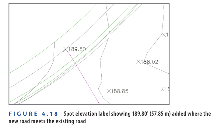
The top-right viewport is zoomed in to the north end of the project near the location where the magenta centerline meets the centerline of the existing road. Your task is to label the elevation of the existing road where these two centerlines meet. - Click one of the contours to select the surface, and then click Add Labels ➢ Add Surface Labels on the ribbon.
- In the Add Labels dialog box, select Spot Elevation as the label type.
- Verify that the spot elevation label style is set to Elevation Only – Existing and the marker style is set to Spot Elevation.
- Click Add. Snap to the northern endpoint of the magenta centerline.
A label is placed at the location you selected (see Figure 4.18).
6: Pan to the south where the road centerline bends at a 90-degree angle.
Note the steep slope to the south of the road in this area. You want to measure and label the slope in this area to determine whether homes can be built here and/or if guardrails will be required for the road.
7: If the Add Labels dialog box is already open, skip to the next step. If not, click one of the contours to select the surface, and then click Add Labels ➢ Add Surface Labels on the ribbon.
8: For Label Type, select Slope.
9: Verify that Slope Label Style is set to Percent-Existing, and click Add.
10: When prompted at the command line, press Enter to accept the default of <One-point>.
11: Click a point to the south of the road to label the slope. Press the Esc key to end the command.
12: Click the label, and then click the square grip at the midpoint of the arrow. Move your cursor across the drawing, and note how the label changes.
13: If the Add Labels dialog box is already open, skip to the next step. If not, click one of the contours to select the surface, and then click Add Labels ➢ Add Surface Labels on the ribbon.
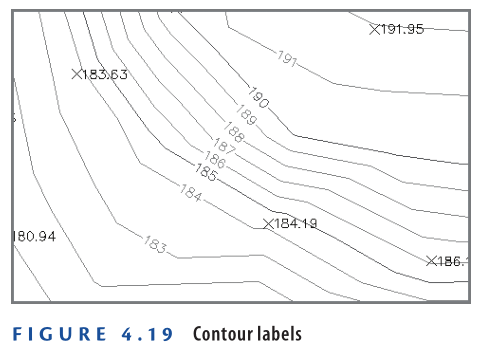
14: For Label Type, select Contour – Multiple. Verify that the names of all three label styles begin with Existing, and click Add.
15: Click two points in the drawing that stretch across several contours.
Contour labels appear where contours fall between the two points you’ve selected (see Figure 4.19).
You’ve actually drawn an invisible line that intersects with the contours
16: Press Esc to clear the previous command, and then click one of the newly created labels.
Notice the line that appears. Click one of the grips, and move it to a new location to change the location of the line. The contour labels go where the line goes, even if you stretch it out and cause it to cross through more contours, in which case it will create more labels.
17: Continue placing contour labels until you’ve evenly distributed labels throughout the drawing.
18: Save and close the drawing.
You can view the results of successfully completing this exercise by opening Labeling Surfaces – Complete.dwg.
https://www.mediafire.com/file/5xtktqyquvx9emq/Labeling+Surfaces+-+Complete.dwg/file
Watch Complete video here for Exercise:
Now You Know
Now that you have completed this chapter, you understand the role of surfaces in land-development projects. You can create surfaces from survey data and perfect them by adding breaklines and boundaries. You can modify surfaces by deleting lines and editing points. You can get answers and tell stories about surfaces using analysis types such as elevation banding, slope banding, and slope arrows. Finally, you’re able to provide additional information about a surface using several different types of labels.
Now that you’ve learned this major step in establishing the existing conditions of your project, you’re ready to begin learning about the tools used to transform your project through design.
Chapter-4 All Exercise: