Combining Design Surfaces
In Chapter 17, you created a pond design that resulted in a surface representing the shape of the pond. You also performed some lot grading, and with continued effort, you would have completed the lot grading for the entire site, resulting in a surface covering most of the project.
In Chapter 9, “Designing in 3D Using Corridors,” you created a corridor surface to represent the road model. This method of designing terrain in segments is common and recommended. Even experienced designers find it more effective to divide the design into parts—such as roads, lots, and ponds—before assembling the full design.
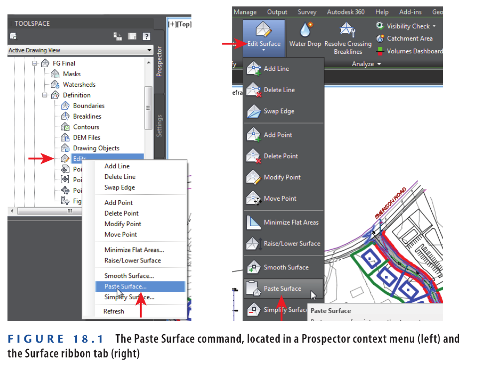
Once all parts are completed, they need to be merged into a master surface. Civil 3D 2025 allows this using the powerful surface pasting feature. Similar to pasting text into a document, you can paste one surface into another. However, unlike text, the pasted surface remains a live reference—any changes to the original surface automatically reflect in the pasted one. To paste surfaces, right-click Edits in a surface under Prospector, or use the Surfaces tab on the ribbon.
Managing Multiple Pasted Surfaces
When working with multiple pasted surfaces in Civil 3D 2025, the paste order plays a key role in achieving the correct final result. If two surfaces overlap, the surface pasted later will overwrite the earlier one in the overlapping areas.
You can control the paste order on the Definition tab of the Surface Properties dialog box. This interface allows you to rearrange the sequence of operations, not only for pasted surfaces but also for other surface edits and definitions (see Figure 18.2). This gives you flexibility in managing how different surface elements interact within your final composite surface.
Exercise 18.1: Combine Surfaces
In this exercise, you’ll create an FG Final surface by combining surfaces that represent lot grading, road elevations, pond grading, and a small daylighting area.
- Open the drawing named Combining Surfaces.dwg which you can download from Video description below.
The lot grading is complete, shown by blue, red, and green feature lines. A grading group was used to calculate daylighting between lots 73 and 76. - In Prospector, expand Surfaces, then right-click Surfaces and choose Create Surface.
- In the Create Surface dialog:
- Set Name to
FG Final - Select Contours 1′ and 5′ (Design) or Contours 0.5m and 2.5m (Design) as the style
- Click OK
The FG Final surface is now listed in Prospector.
- Set Name to
- Expand Surfaces ➢ FG Final ➢ Definition. Right-click Edits and select Paste Surface.
- In the Select Surface To Paste dialog, choose
Lots – Exterior, then click OK.
Contours for the exterior lots appear in the left viewport. The bottom-right viewport displays the 3D model of interior grading. - In the left viewport, zoom in to the interior lot area. Notice the irregular contours extending across the road.
- Click any red or blue contour to select the surface. Then on the ribbon, click Edit Surface ➢ Paste Surface.
- Select
Road FG, then click OK.
Contours in road areas now match the correct road elevations. The 3D model shows defined curbs and road crowns. The interior lot area is empty due to a hide boundary in the Road FG surface. - Repeat step 7–8, selecting the
Pondsurface. - Repeat step 7–8 again, this time selecting the
Lots – Interiorsurface. - Click a contour again, and on the ribbon, select Surface Properties.
- In the Surface Properties dialog:
- Go to the Definition tab
- Click Add Surface Lots – Interior
- Use the up-arrow icon to move
Lots – InteriorabovePondin the paste order (see Figure 18.3).
This completes the combination of all surfaces into the FG Final surface in Civil 3D 2025
- Click OK, then click Rebuild The Surface.
Now the surface displays accurate lot grading contours along with the correct pond contours.
This demonstrates how essential it is to manage the paste order of surfaces to get the desired design output. - Repeat steps 7 and 8, this time selecting the
Lot Daylightsurface.
Contours now appear in the area between lots 73 and 76, completing the design.
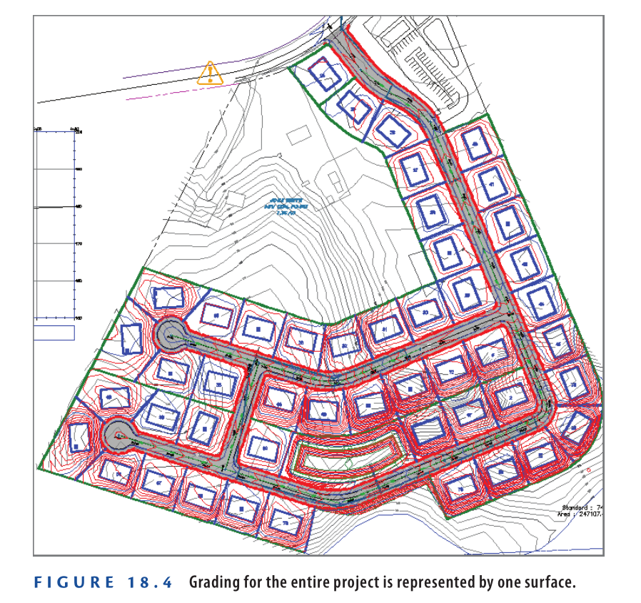
All grading elements of the project are now merged into a single, unified surface (see Figure 18.4).
- Save and close the drawing.
You can view the results of successfully completing this exercise by opening Combining Surfaces – Complete.dwg.
https://www.mediafire.com/file/1aexeduuy0ferrj/Combining+Surfaces+-+Complete.dwg/file
Watch Video Tutorial here for this Exercise:
Modular Design
In the previous exercise, you observed five design surfaces listed in Prospector, each representing a separate mini-design. These surfaces originate from different parts of the project and follow a modular design approach.
Lots – Exterior
This surface was created using feature lines that define the grading for all lots except those located between Jordan Court, Madison Lane, and Logan Court. These feature lines were added to the Lots – Exterior surface as breaklines.
To define the boundary, a polyline was drawn along the back edges of the lots and added as an outer boundary. The surface was then allowed to triangulate over the road and interior lot areas, filling in those gaps temporarily.
The 3D view clearly shows how the Lots – Exterior surface forms part of the complete grading model.
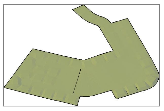
Lots – Interior
This surface was created using feature lines that define the grading for all lots enclosed between Jordan Court, Madison Lane, and Logan Court. These feature lines were added to the Lots – Interior surface as breaklines.
A polyline was drawn along the front edges of the lots and added as an outer boundary. The surface was then allowed to triangulate across the pond area to complete the surface temporarily.
The 3D representation shows how the Lots – Interior surface fits within the overall site model, forming a detailed section of the complete grading design.
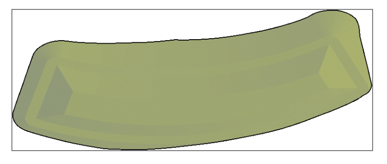
Pond This surface is created from the grading group used to design the pond south of lots 69 and 70. The following image shows the Pond surface in 3D.
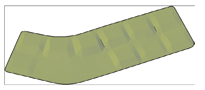
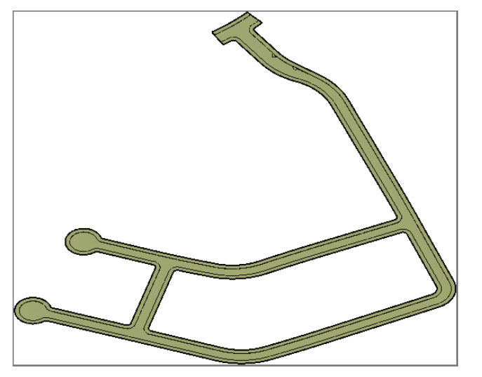
Road FG This surface is created from the road corridor. The following image shows the Road FG surface in 3D view.
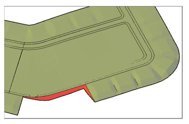
lot Daylight This surface is created from a grading group used to design the daylighting between lots 73 and 76. It’s shown in the following graphic in red along with the Road FG surface and Lot – Exterior surface in tan.
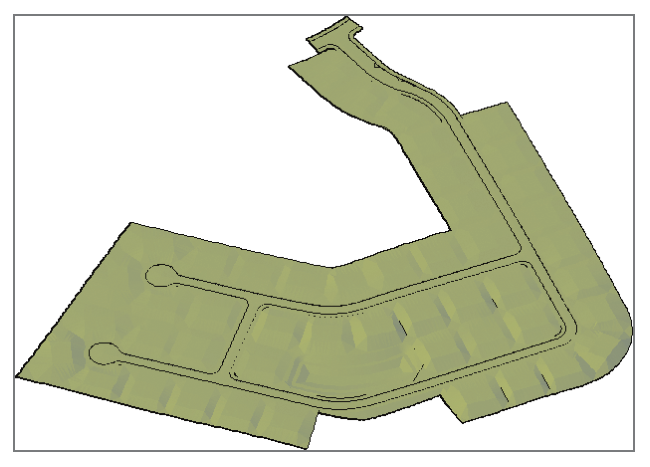
In the preceding exercise, you combined all these surfaces to create a single finished ground surface, as shown in 3D view in the following image.
Analyzing Design Surfaces
Civil 3D 2025 offers much more than just contour display when working with surfaces. While it’s not possible to cover every capability in one section, this part focuses on some of the most commonly used surface analysis features, grouped into three key categories: surface analysis, hydrology tools, and quick profiles.
Using Surface Analysis
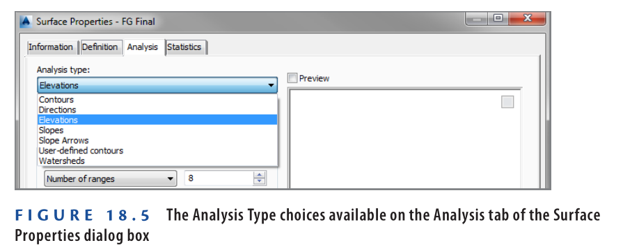
In this context, surface analysis refers to the tools found on the Analysis tab of the Surface Properties dialog box. Here, you can conduct detailed evaluations related to elevations, slopes, contours, and watersheds (see Figure 18.5).
The analysis results are displayed graphically in your drawing. Depending on the type of analysis, these may appear as:
- Shaded regions
- Directional arrows
- Color-coded contour lines
- 3D-rendered zones
To enhance clarity, you can also create a legend that explains the meaning of each color, making your analysis easier to interpret and communicate.
Analyzing a surface involves two main steps. First, use the Surface Properties dialog box to create analysis ranges. This step does not affect the drawing visually but generates the data needed for graphical output. Second, apply a surface style that displays the analysis components. For instance, to view slope arrows, you must define slope ranges and then apply a surface style that shows slope arrows.
Exercise 18.2: Analyze Surfaces
This exercise guides you through performing a slope analysis to highlight steep areas in your project. You’ll also modify a lot to show how analysis supports design decisions.
- Open the file named Analyzing Surfaces.dwg which you can download from video description below.
- Click a red or blue contour in the drawing, then select Surface Properties from the ribbon.
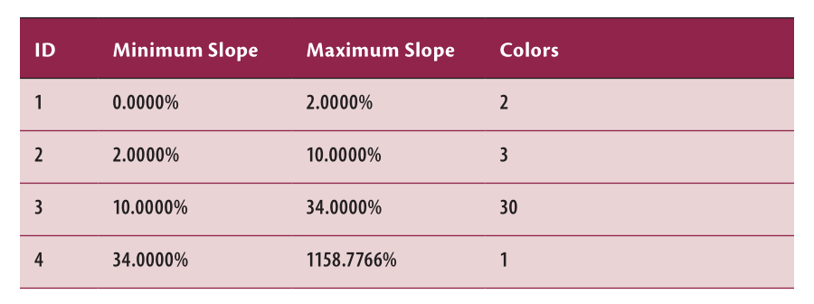
- In the Surface Properties dialog, go to the Analysis tab. Choose Slopes as the analysis type. Set Number of Ranges to 4.
- Click the Run Analysis icon (downward arrow). Four ranges will appear in the Range Details section.
- Adjust the slope ranges as needed.
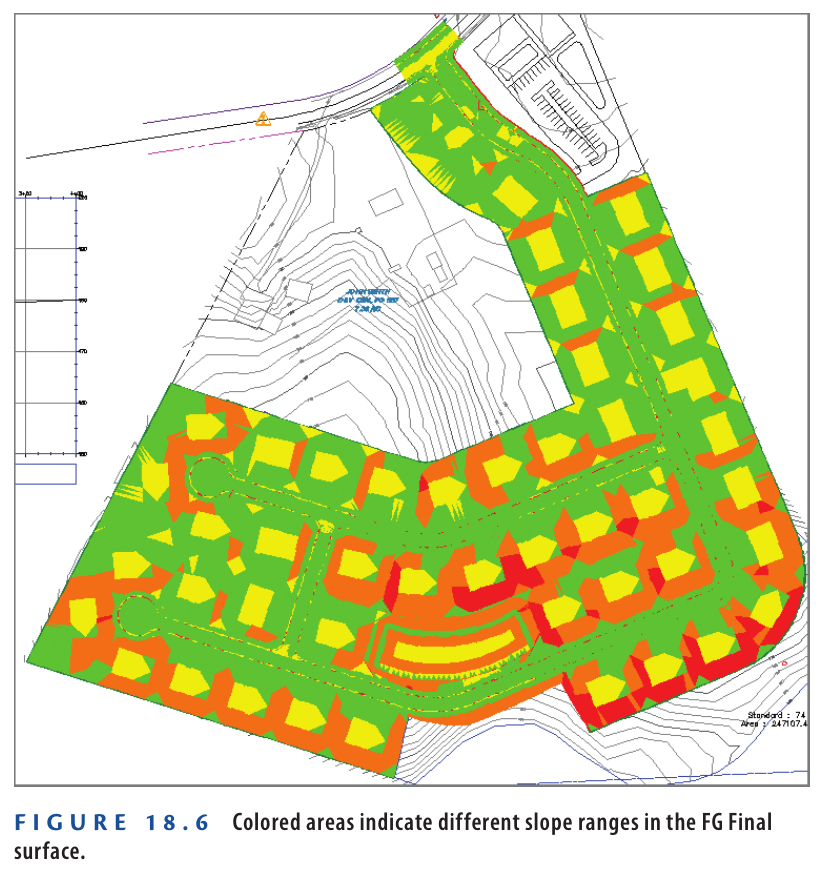
- Go to the Information tab and change the style to Slope Banding (2D). Click OK, then press Esc to deselect the surface.
The drawing now shows colored areas representing slope categories: yellow for flat slopes (0%–2%), green for moderate slopes (2%–10%), orange for steep slopes (10%–34%), and red for very steep slopes (>34%). - Click one of the colored areas to select the surface. Right-click and choose Display Order ➢ Send To Back.
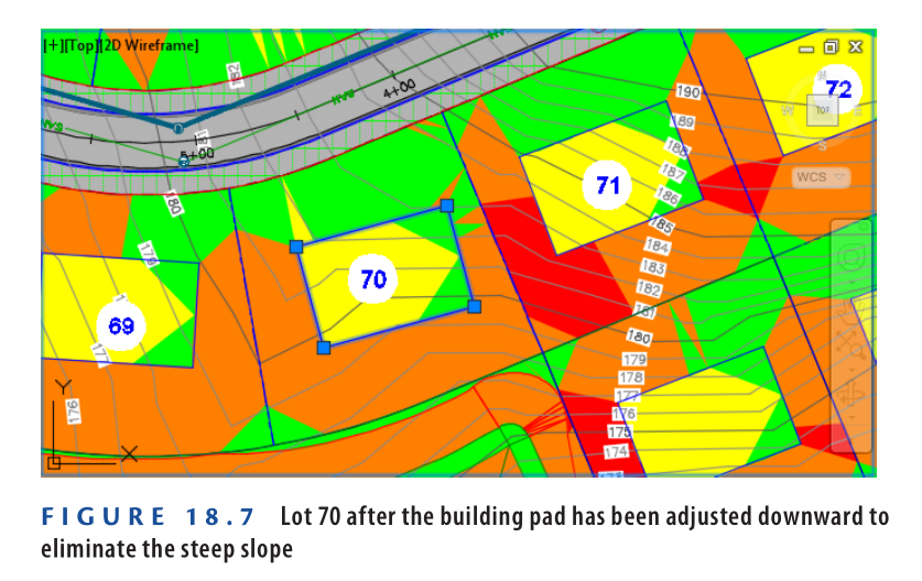
- Press Esc to clear the selection. In the top-right viewport, click the blue rectangular feature line at the center of Lot 70. On the ribbon’s Edit Elevations panel, click Raise/Lower.
- At the command line, enter -5 ( -1.524 ) for the elevation difference, then press Enter.
After a short pause, the surface rebuilds. The red area in Lot 70 disappears. The front yard stays green, indicating it’s within a suitable slope range for driveway installation.
- Save and close the drawing.
You can view the results of successfully completing this exercise by opening Analyzing Surfaces – Complete.dwg.
https://www.mediafire.com/file/xnlycgd5bh7hn9x/Analyzing+Surfaces+-+Complete.dwg/file
Watch Complete Video here for this Exercise:
Using Hydrology Tools
Civil 3D 2025 provides two powerful tools for analyzing surface drainage: Water Drop and Catchments. The Water Drop tool simulates the path of a raindrop flowing downhill from a selected point, helping identify flow direction and low spots where water accumulates. The Catchments tool defines the drainage area that flows toward a specific point, useful for designing stormwater systems like inlet sizing.
Exercise 18.3: Analyze Hydrology
- Open the drawing Using Hydrology Tools.dwg which you can download from Video tutorial description below.
- Go to the Analyze tab, then click Flow Paths ➢ Water Drop.
- When prompted, press Enter to choose a surface from a list.
- In the Select A Surface dialog, choose EG-FG Composite and click OK.
- In the Water Drop dialog, click OK, then click a point in lot 29 near the road. A blue flow path appears toward the inlet near station 2+50 (0+080).
- Click another point near the southeast corner of lot 23.
- Press Esc, then click Catchments ➢ Create Catchment From Surface.
- Choose the center of the red circle at the end of the second flow path.
- In the dialog, set EG-FG Composite as the surface and click OK. A blue outline shows the catchment draining to the selected inlet.
- Save and close the drawing. To verify results, open Using Hydrology Tools – Complete.dwg.
https://www.mediafire.com/file/onwmjp4n4qe99be/Using+Hydrology+Tools+-+Complete.dwg/file
Watch Complete Video Tutorial here for this Exercise:
Using a Quick Profile
Civil 3D 2025’s Quick Profile tool creates temporary profiles from lines, arcs, polylines, or feature lines. These profiles help visualize the relationship between existing and proposed surfaces without requiring full alignment-based profiles. They update with any changes to the original object but disappear upon saving.
Exercise 18.4: Analyze Using a Quick Profile
- Open Using a Quick Profile.dwg which you can download from video Tutorial description below.
- In the left viewport, locate the thick red polyline that cuts across the pond.
- Go to the Analyze tab and click Quick Profile.
- Select the red polyline when prompted.
- In the dialog, uncheck Select All Surfaces, then check EG and FG Final. Set FG Final to use the Design Profile style.
- Click OK, then click in the lower-left corner of the upper-right viewport. A profile view appears, showing existing ground (red) and proposed ground (black). Notice the pond’s shape and nearby road formations in the profile (see Figure 18.8).

- Click the red polyline to reveal its grips. Select any grip and move it to a new location.
- Press Esc to deselect the polyline. Zoom into the interior lots, and find the green feature line forming the back boundaries of lots 68–70.
- On the Analyze tab, click Quick Profile. When prompted, select the green feature line identified earlier.
- In the Create Quick Profiles dialog, check the box for EG. Ensure the Draw 3D Entity Profile option is checked. Set the 3D Entity Profile Style to Design Profile.
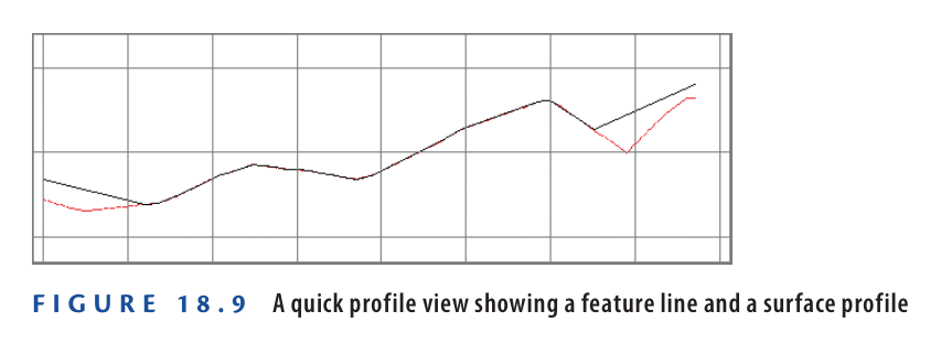
- Click OK, then click a point to the right of the existing profile view. A new profile view appears, showing existing ground in red and the feature line in black. Observe how the feature line closely follows existing ground, except at both ends where it connects to finished elevations (see Figure 18.9).
- Save and close the drawing.
You can view the results of successfully completing this exercise by opening Using a Quick Profile – Complete.dwg . Note that the “Complete” version of the file isn’t much different from the original because quick profiles are removed when the drawing is saved.
https://www.mediafire.com/file/pqg2lhcrl4nsrs0/Using+a+Quick+Profile+-+Complete.dwg/file
Watch Complete Video Tutorial here for this Exercise:
Calculating Earthwork Volumes
Earthmoving is one of the most costly activities in land development projects. Two key questions must be addressed in nearly every grading design:
▶▶ How much earth needs to be moved?
▶▶ How much material must be imported or exported from the site?
As an engineer or designer, your goal is to minimize these volumes. Reducing earth movement lowers construction costs and benefits the client or property owner. Importing or exporting soil is particularly expensive, so minimizing this also reduces environmental and financial impact.
Understanding Earthwork Volumes
Earthwork involves two main operations: cut and fill.
- Cut refers to soil removed from the ground.
- Fill refers to soil added to the ground.
Each excavation (cut) and each deposit (fill) adds up to final earthwork quantities. If cut and fill values are equal, the project is called a balanced site—meaning no soil needs to be transported in or out. Achieving this balance saves money and minimizes site disruption. It’s a standard goal for civil engineers in grading design.
Using the Volumes Dashboard
Civil 3D 2025 offers several tools for calculating earthwork, but the Volumes Dashboard is a primary feature. Located on the Analyze tab, the Volumes Dashboard opens in the Panorama window.
You can:
- Add or create TIN volume surfaces
- View cut and fill results
- Create bounded volumes for smaller areas like lots or project phases
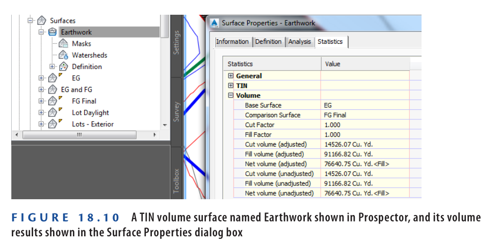
- Generate detailed volume reports in your browser or directly within Civil 3D (see Figure 18.10)
Exercise 18.5: Analyze Earthwork
In this exercise, you’ll use the Volumes Dashboard in Civil 3D 2025 to analyze cut and fill volumes for the full site and three specific lots.
- Open the drawing Calculating Volumes.dwg which you can download from video Tutorial description below.
- Go to the Analyze tab, then click Volumes Dashboard.
- In the Volumes Dashboard tab of Panorama, click Create New Volume Surface. In the dialog box:
a. Set Name to Earthwork
b. Set Style to No Display
c. Set Base Surface to EG
d. Set Comparison Surface to FG Final
e. Click OK The cut and fill values are now shown in Panorama. The Fill Volume is significantly higher than the Cut Volume, indicating the project is not balanced. More fill is required, meaning additional soil will need to be brought in. You can reduce this need by adjusting grading—such as lowering building pads or profile elevations—to increase cut and reduce fill. - Click the Earthwork entry, then select Add Bounded Volume. When prompted, click the parcel label for Lot 1.
- Repeat this step for Lots 2 and 3. Click the plus (+) sign beside Earthwork to expand the volume list.
- Rename Earthwork.1 to Lot 1, Earthwork.2 to Lot 2, and Earthwork.3 to Lot 3.
Check the boxes beside each lot and click Generate Cut/Fill Report.
Your browser opens with a detailed earthwork report for the entire site and all three lots. - Save and close the drawing. To verify results, open Calculating Volumes – Complete.dwg and open the Volumes Dashboard.
https://www.mediafire.com/file/3wjf6e2538j2euf/Calculating+Volumes+-+Complete.dwg/file
Watch Complete Video Tutorial here for this Exercise:
What Is a TIN Volume Surface?
TIN stands for Triangular Irregular Network, a method of forming surfaces using 3D point data connected into triangles. A TIN surface is built from these triangles to represent terrain.
A TIN volume surface is created by superimposing one TIN surface (such as proposed grading) over another (such as existing ground). Civil 3D calculates the elevation differences at intersecting triangle points, then generates a new surface from those differences. These represent:
- Cut (negative values): Material to be removed
- Fill (positive values): Material to be added
Other Volume Methods
In addition to the Volumes Dashboard, Civil 3D 2025 supports three other volume calculation tools:
- TIN Volume Surface: Can be created using the Create Surface command by selecting TIN Volume Surface. Results are viewed under Surface Properties > Statistics tab.
- Grading Volume Tools: Used with grading groups that reference a volume base surface. These tools can calculate, adjust, and even balance grading designs.
- Quantity Takeoff Criteria: Generates section-based volume calculations using a sample line group. This is typically used in corridor models for transportation design.
Labeling Design Surfaces
As with all other design types covered in this book, surface designs must be annotated. The information conveyed through labeling is nearly as critical as the design itself, especially when it comes to grading.
From a documentation perspective, the main deliverable in a grading design is a set of design contours. However, contours alone don’t provide sufficient construction guidance. Once labeled, they help contractors understand exactly how to shape the land according to the design intent. In some cases, labels are needed to show specific elevations and slopes. These are known as spot elevations or spot grades when referring to a single point’s elevation.
Although it was discussed earlier, you previously learned to create contour, spot, and slope labels in Chapter 4. You’ll now apply those skills again—this time for proposed, not existing, elevations.
Exercise 18.6: Label a Design Surface
In this exercise, you’ll create contour, spot elevation, and slope labels for lot 2 and use them to refine the design.
- Open the drawing named Labeling Design Surfaces.dwg which you can download from video Description below.
- Go to the Annotate tab on the ribbon and click Add Labels.
- In the Add Labels dialog box:
a. For Feature, choose Surface.
b. For Label Type, select Contour – Multiple.
c. Click Add. - When prompted to select a surface, click on one of the red or blue contours in the drawing.
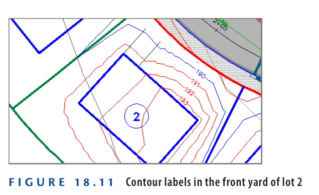
- When asked to specify the first point, pick two points that create a line through the contours in the front yard of lot 2 (refer to Figure 18.11).
- In the Add Labels dialog box, change the Label Type to Contour – Single. Click Add.
- When prompted to select a surface, click on one of the red or blue contours in the drawing.
- Click on several contours across the Jordan Court road surface to label them individually.
- In the Add Labels dialog box, change the Label Type to Slope. Click Add.
- When prompted to select a surface, click any red or blue contour to select the surface.
- When prompted to choose between One-Point and Two-Point labeling, press Enter to select One-Point. Pick a point near the center of the front yard of lot 2.
The slope label will show that the grade in this area exceeds the allowable 10%. You’ll fix this later in the exercise. - In the Add Labels dialog box, change the Label Type to Spot Elevation.
- Click Add, and when prompted to select a surface, click any red or blue contour.
- Using the Endpoint object snap, select all four corners of the lot 2 building pad. This will place spot elevation labels at each corner.
- Press Esc to exit the labeling command. Click on the blue building pad feature line for lot 2. On the Edit Elevations panel of the ribbon, click Raise/Lower.
- When prompted to specify the elevation difference, type
-2(or-0.691) and press Enter.
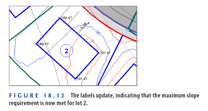
After a brief surface rebuild, all contour, slope, and spot elevation labels will update to reflect the elevation change (see Figure 18.12). The slope in the front yard of lot 2 will now be within the allowed 10%.
- Save and close the drawing.
You can view the results of successfully completing this exercise by opening Labeling Design Surfaces – Complete.dwg.
https://www.mediafire.com/file/xt7b7jvemcg2zxz/Labeling+Design+Surfaces+-+Complete.dwg/file
Watch Complete Video Tutorial here for this Exercise:
The New Way to Build
While contours remain the most common output of a design surface, new technologies are transforming how grading designs are used. One of the fastest-growing methods is the machine model. Contractors now utilize GPS-guided excavation equipment that syncs with computer-generated models representing the design layout.
Where does this model originate? From Civil 3D and similar tools. Although contractors typically review and refine the model before deploying it in the field, it all begins with the grading design created in Civil 3D. A clean, accurate finished ground surface leads directly to a more precise and efficient construction process.
Now You Know
After completing this chapter, you’ve learned how to build a grading design in segments and combine them using surface pasting. You know how to analyze surfaces and make data-driven adjustments. You’ve practiced applying slope, hydrology, and earthwork analysis to real-world scenarios.
Most importantly, you can now label your design surface—a critical step that both communicates essential information and helps identify and resolve design problems.
You’re now prepared to start compiling, analyzing, and labeling design surfaces in a real production workflow.